High quality plots for LaTex with PGF-Tikz and Gnuplot
PGF-Tikz enables the creation of high quality drawing for LaTex. An example of script is present here to create a plot by exploiting both the quality of Tikz and the power of Gnuplot.
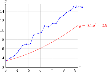
This figure has been generated using the following LaTex script figure.tex.
\documentclass{article}
\usepackage{tikz}

\begin{document}
\pagestyle{empty}

\begin{tikzpicture}[x=1cm,y=0.4cm]

  \def\xmin{3}
  \def\xmax{9.2}
  \def\ymin{2}
  \def\ymax{15.5}

  % grid
  \draw[style=help lines, ystep=2, xstep=1] (\xmin,\ymin) grid
  (\xmax,\ymax);

  % axes
  \draw[->] (\xmin,\ymin) -- (\xmax,\ymin) node[right] {$x$};
  \draw[->] (\xmin,\ymin) -- (\xmin,\ymax) node[above] {$y$};

  % xticks and yticks
  \foreach \x in {3,4,...,9}
    \node at (\x, \ymin) [below] {\x};
  \foreach \y in {2,4,...,14}
    \node at (\xmin,\y) [left] {\y};

  % plot the data from the file data.dat
  % smooth the curve and mark the data point with a dot
  \draw[color=blue] plot[smooth,mark=*,mark size=1pt] file {data.dat}
   node [right] {data};

  % generate and plot another a curve y = 0.1 x^2 + 2.5
  % this generates the files figure.parabola.gnuplot and figure.parabola.table
  \draw[color=red, domain=\xmin:\xmax] plot[id=parabola]
  function{0.1*x**2 + 2.5} node [right] {$y=0.1\,x^2 + 2.5$};

\end{tikzpicture}

\end{document}
The data contained in the following file data.dat are plotted.
3.045784        3.415896
3.405784        4.025693
3.785784        4.522530
4.125784        5.538449
4.485784        6.704992
4.805784        6.978939
5.145784        7.113496
5.425784        8.916397
6.065784        9.487712
6.365784        10.876397
6.685784        10.693497
7.025784        11.364131
7.345784        11.442530
7.665784        12.582530
8.005784        13.125693
8.225784        13.738450
8.585784        14.247891
8.865784        14.982530
This file can be compiled by the command
pdflatex --shell-escape figure.tex
The option "--shell-escape" is necessary to allow the execution of Gnuplot. Once this file had been compiled, it creates two more files: "figure.parabola.gnuplot" and "figure.parabola.table". The first one contains the gnuplot script which create the parabola and the second one the points of this parabola. Thus, the second time the LaTex file "figure.tex" is compiled, the data in the file "figure.parabola.table" are read and Gnuplot is not executed a second time. Here are displayed the content of the files "figure.parabola.gnuplot" and "figure.parabola.table".
set terminal table; set output "figure.parabola.table"; set format "%.5f"
set samples 25; plot [x=3:9.2] 0.1*x**2 + 2.5
#Curve 0, 25 points
#x y type
3.00000 3.40000  i
3.25833 3.56167  i
3.51667 3.73669  i
3.77500 3.92506  i
4.03333 4.12678  i
4.29167 4.34184  i
4.55000 4.57025  i
4.80833 4.81201  i
5.06667 5.06711  i
5.32500 5.33556  i
5.58333 5.61736  i
5.84167 5.91251  i
6.10000 6.22100  i
6.35833 6.54284  i
6.61667 6.87803  i
6.87500 7.22656  i
7.13333 7.58844  i
7.39167 7.96367  i
7.65000 8.35225  i
7.90833 8.75417  i
8.16667 9.16944  i
8.42500 9.59806  i
8.68333 10.04003  i
8.94167 10.49534  i
9.20000 10.96400  i
Nevertheless, the generated PDF file is a whole page. So, PDFcrop can be used.
pdfcrop figure.pdf figure.pdf
Then, the PDF plot can be converted to a PNG image using ImageMagick.
convert -density 96 -units PixelsPerInch figure.pdf figure.png
This create a PNG image with 96 DPI (Dots Per Inch). This is the
standard resolution for screen display. For a LaTex paper, it is
recommended to keep the PDF file or to use a resolution of at least
300 DPI for color graphics and 6OO DPI for black and white
graphics.
The whole process is automated by the following BASH script.
#!/bin/bash

for file in *.tex
do
    echo "Processing $file ...";
    pdflatex --shell-escape $file
    pdfcrop ${file%.tex}.pdf ${file%.tex}.pdf
    convert -density 96 -units PixelsPerInch ${file%.tex}.pdf ${file%.tex}.png
done
At last, the created plot can be included very simply in a LaTex document.
\begin{figure}
    \includegraphics{figure1.pdf}%
    \hfill%
    \includegraphics{figure1.png}
\end{figure}
And the figure is included at the good size.
That's all folks!
